Stacking Fault
Simulations – I
In this exercise you will use GSAS-II to simulate the diffraction patterns from faulted diamond. Diamond most commonly has the well-known cubic structure with the space group Fd3m and a=3.5668A. The C-atom is at 1/8,1/8,1/8 and can be viewed as a cubic stacking of ruffled hexagonal nets along the cubic cell 111 diagonal.
The structure of londsdaleite has those layers stacked hexagonally and thus a faulted diamond structure may occasionally have hexagonal stacked layers instead of all cubic ones. From geometric considerations, these planar stacking faults must extend across the entire crystal. If there are only a few such faults in a crystal then the diffraction pattern will show two cubic diamond patterns in a twin law relationship. Otherwise, if there are many such faults then the diffraction pattern will show streaks. To simulate the streaks one must first develop a model for the hexagonal net of C-atoms and then show how they stack in either the cubic or hexagonal forms. GSAS-II uses a suite of subroutines from the DIFFaX program (M.M.J. Treacy, J.M. Newsam & M.W. Deem, (1991), Proc. Roy. Soc. Lond. 433A, 499-520) to calculate the diffraction pattern via a general recursion algorithm and a randomized set of stacked layers. NB: this calculation can be quite time consuming particularly if unreasonable demands are made on it.
If you have not done so already, start GSAS-II.
Simulation 1.
Selected area diffraction for random faults in diamond
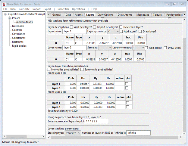
To begin we must have a phase to work with. In the main GSAS-II data tree menu do Data/Add new phase; a popup window will appear inviting you to name the phase. I entered ‘random faults’. Then find this phase in the data tree under phases and select it; the data window will display the default for the General tab.
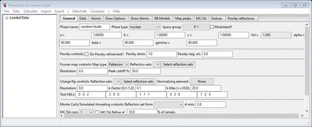
Change the phase type to ‘faulted’; the window will be redrawn and a new tab (‘Layers’) will appear. Select it. Then save the project; I called it ‘diamond’.
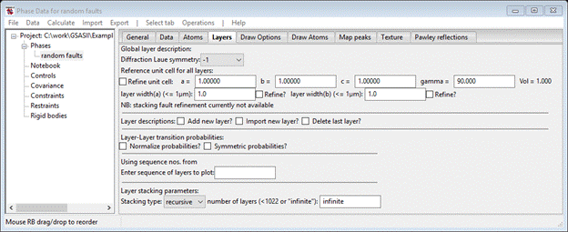
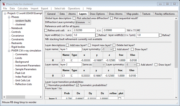
First you need to describe the reference unit cell for the stacking model. The cubic/hexagonal stacking in diamond is with layers perpendicular to the 111 axis. This will become the new c-axis. The a- & b-axes are for the hexagonal net of C-atoms that are stacked in this structure. One can also anticipate that the resulting diffraction pattern will have hexagonal 6/mmm symmetry so first select this from the pull down box near the top of the page; the window will be redrawn.

The a cell parameter for diamond
stacking can be assumed to be ![]() =
2.522 and the c
cell parameter is
=
2.522 and the c
cell parameter is ![]() =
2.059 since there
are 3 layers along the 111 diamond cell diagonal. Enter these in the
appropriate places; the cell volume will be revised.
=
2.059 since there
are 3 layers along the 111 diamond cell diagonal. Enter these in the
appropriate places; the cell volume will be revised.
Now we have to describe the two hexagonal nets that will be stacked for either cubic or hexagonal stacking. Select Add new layer? the window will be redrawn.

Name the layer (I chose ‘layer 1’) and choose ‘-1’ for the layer symmetry. The window will be redrawn after changing the name. Next, select Add atom? and the window will be redrawn with one line in the layer table.
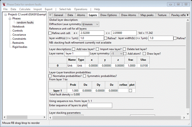
To make this a C-atom select the ‘Unk’ under Type with a double click; a Periodic table will popup. Select C; the popup will disappear and the window will be redrawn. The coordinates of this C-atom in the new stacking unit cell is -1/3,-1/6,-1/8; you may enter these as fractions. Select a table item to complete the entry; the window should show the new position.
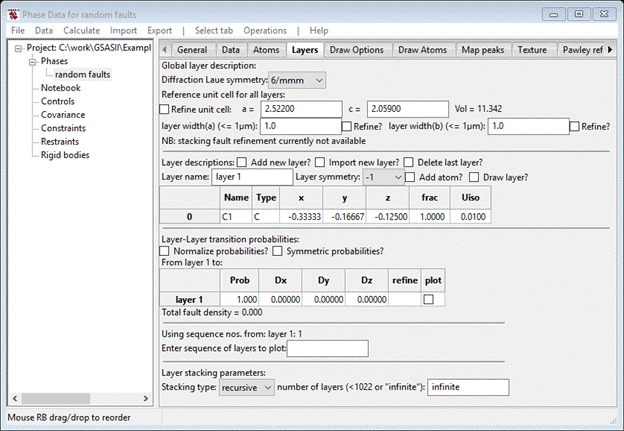
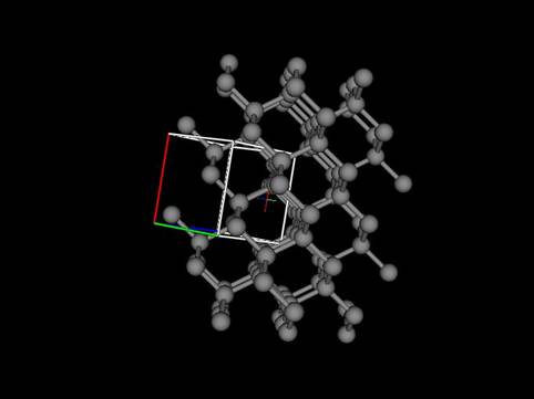
You can draw the layer to see what it looks like; select Draw layer? and the drawing will appear.
A unit cell box is drawn with a 5x5 suite of unit cells; the ruffled hexagonal net perpendicular to the c-axis (blue line) is clear.
Now we need a second layer (‘layer 2’); repeat the steps for making a layer using 1/3,1/6,-1/8 for the C-atom position with -1 for the layer symmetry. The window should look like this when done.

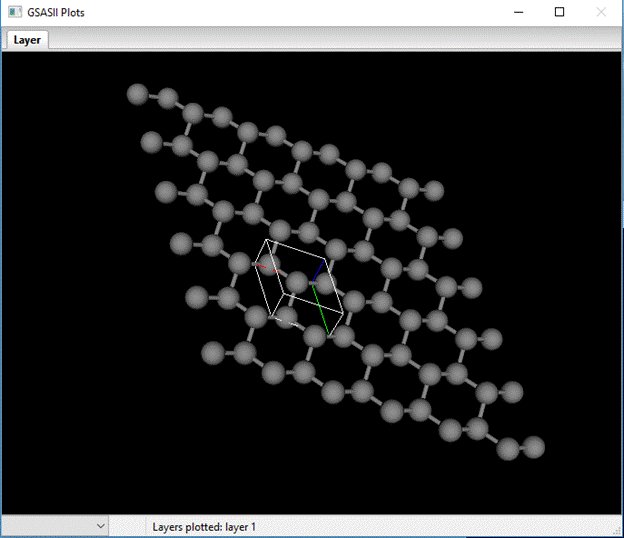
I’ve stretched it a bit to show the Layer-Layer transition probabilities. Change Dz for each entry to 1.0 to properly space out the stacked layers. If you select the first box in the plot column for layer 1 you will see the two layers stacked but in a way reminiscent of how carbon sheets stack in graphite.
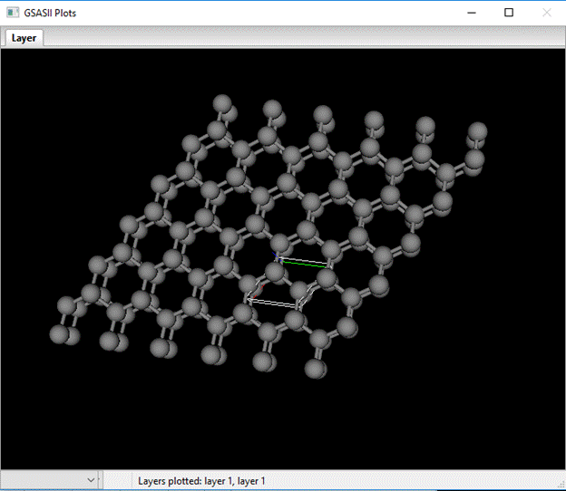
Clearly not diamond stacking. The table defines how the next layer is displaced relative to the reference layer. You can shift this layer by using the X,Y,Z & shift-X,Y,Z keys; the plot will be redrawn and the table entry updated each time you shift the layer. When you get to the right offset for diamond additional bonds will appear connecting the layers together. The correct shift is Dx=2/3, Dy=1/3 and Dz=1.0 for the layer 1 to layer 1 transition and for layer 2 to layer 2 the shifts are Dx=-2/3, Dy=-1/3 and Dz=1.0. For the remaining layer 1-layer 2 and vice versa transitions Dx=Dy=0. Layer 1 to layer 1 stacking looks like.
You can explore the result of various stacking sequences in the next block of commands; enter 1 1 1 1 2 2 2 into the box (remember to include spaces in between each number) and press Enter. A plot showing the result of a single twin fault will be shown.

If you enter 1 2 1 2 1 2 1 2 then the structure of londsdaleite will be shown; 1 1 1 1 1 1 or 2 2 2 2 2 2 gives the diamond structure.
Finally we must select transition probabilities; they should sum to 1.0 for each block. Use 0.7 for layer 1 to layer 1 and layer 2 to layer 2; the cross terms are then 0.3 to give
We are now ready to do a single crystal simulation; select Operations/Simulate pattern from the Phase data window menu. A small popup will appear
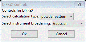
Select selected area for the calculation type; the popup will be redrawn with new options.
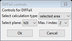
To make it interesting select Max. l index of 6 and press Ok. Very quickly a new popup will appear letting you know the simulation is finished; press Ok. The data window will be redrawn

At the top is a new item Plot selected area diffraction? Select it and a new plot will appear. The intensity scale is adjusted by pressing D (or U); I got

The streaking intermixed with sharp spots is clearly obvious in this plot. Save this project; you’ll need it for the next simulation.
Simulation 2.
Laboratory powder diffraction simulation for random faults in diamond
The setup for a powder pattern simulation is the same as above for selected are diffraction with one crucial difference. We need a dummy powder pattern to define the simulation limits. Using the same project as above, do Import/Powder data/Simulate a data set from the main GSAS-II data tree window. A popup will appear requesting the selection of an instrument parameter file; here we will use one of the built in defaults. Press Cancel and a new popup will appear offering some choices.
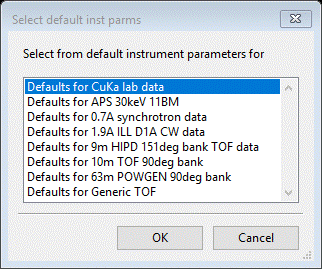
Use the first one for CuKa lab data; a new popup will appear
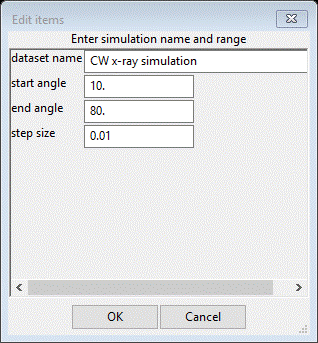
Change the end angle to 150 and the step size to 0.02; press Ok and choose random faults (your phase name). Notice the small data window lets you know that you can clear the observed intensities in the simulation by doing an Edit range (no need to change anything). The tree will have a new item PWDR CW x-ray simulation. Select Background & enter 50 for the 1st coefficient. Next select Sample parameters and enter 1000 for the Histogram scale factor and change the Diffractometer type to Bragg-Brentano (if not already set to that). Finally, find your phase (random faults) and select it and then the Layers tab. It should be unchanged from when the selected area simulation was finished.
To do the simulation do Operations/Simulate pattern and press Ok from the popup. The calculated pattern will by default be broadened using U, V, & W from the Instrument parameters for the chosen powder pattern. Other choices use a mean Gaussian broadening (faster) or no broadening (even faster). The only choice for the pattern is given in the next popup; press Ok and the simulation will proceed. After a few seconds a small popup will appear letting you know it is done; press Ok and the powder pattern will be displayed with the result. On the plot press the ‘+’ key to suppress the ‘+’ marks. The plot should look like:

The blue line is a simulated observed pattern with imposed Poisson noise, the red line is the calculated background and the green curve is the smooth calculated pattern. A difference curve is also shown. You can play with changing the transition probabilities and/or the layer offsets to see what effect these have on the pattern; changing these will change the calculated pattern unless you reset the dummy profile as noted above.
Simulation 3.
Sequential parameter change
A perhaps useful means of exploring the effects of changing stacking parameters is doing a sequence of simulations varying one parameter over a range. To try this out do Operations/Sequence simulations from the Layers menu; a popup will appear
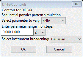
Here you select the parameter, range and number of steps (both ends will be used). From the Select parameter pulldown choose TransP;0;0; this is the layer 1 to layer 1 transition probability. Then change the no. steps to 10 (11 will be calculated). We have the same choices for instrument broadening as above; use the default. Press Ok; the next popup allows selection of a powder pattern (e.g. for comparison and the range for the calculation). Press Ok for this one; the sequential simulation will proceed. The console displays progress and the transition matrix for each step. A popup will appear when the sequence is finished after several seconds. Notice that the matrix is not symmetric (see console) so that layer1 to layer 1 probability is not the same as layer 2 to layer 2 at each step in the simulation. We can force this by selecting Symmetric probabilities? on the Layers tab. Do this and repeat the sequential simulation as above. Now the matrices are symmetric as one could expect. When the simulation is finished, select the Plot sequential result? box; a new plot will appear.

This is a multiline plot; you can shift the lines with the U,D,L,R keys (O resets offsets to zero). I’ve done this for the next plot.
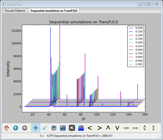
The first blue line is for pure hexagonal londsdaleite stacking and the last magenta line is for pure cubic diamond stacking. You can see how some lines quickly vanish with the introduction of stacking faults while other persist across the entire sequence. This is a good place to save your project file; the sequential result will be included.
Simulation 4.
Modelling clustering in diamond
In this simulation we will explore the possibility that the stacking history affects the probability of a fault. In the case of diamond, a fault to form londsdaleite could be followed by similar layers until a lower probability fault converts the structure back to diamond. The crystal then has blocks of diamond structure interleaved with blocks of londsdaleite. This is best done in a new phase so we don’t mess up the above simulations, but most of the data in the current phase is useful for the cluster model. The easiest way is to import the new phase from the current project. Do Import/Phase/from GSAS-II gpx file from the main GSAS-II data tree menu. A file selection dialog box will appear; select the current project file (diamond.gpx) and press Open. A small popup will appear confirming your choice; press Yes. The next popup offers the change to name the phase, I chose clustered for the name. Next select the PWDR data set to be linked to this phase. The General tab for the new phase will appear.
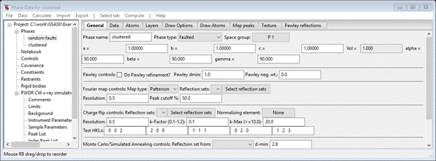
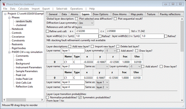
Notice that the Phase type is faulted and that Layers is one of the tabs; select it.
This is all the same information as for the random faults phase. To simulate clustering we need two new layers which are the same as these two listed here. Do Add new layer? twice so two new layers appear. Name them layer 3 and layer 4. Make layer 3 Same as layer 1 (select from the pull down) and layer 4 Same as layer 2. Each time the window is redrawn so that the transition probability tables reflect these changes. You should also change the Diffraction Laue symmetry to -3m. When you are done the upper part of the Layers window should look like.
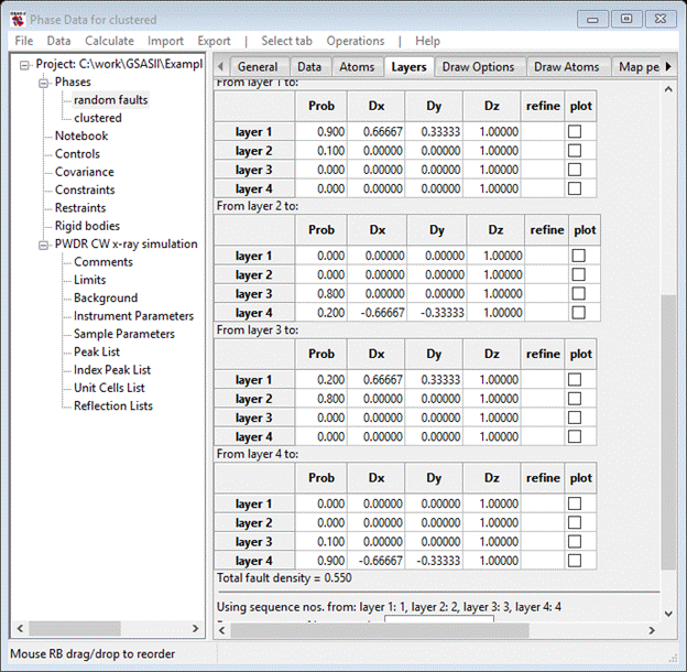
The transition vectors for the cluster model are similar to the random faults model, i.e. layer 1-1 and layer 3-1 transitions are 2/3,1/3,1 for Dx, Dy & Dz, layer, and layer 2-4 and 4-4 transitions are -2/3,-1/3,1 for Dx, Dy & Dz. All the rest are 0,0,1 for Dx,,Dy & Dz. The probabilities can best be seen from the following array
|
Layer |
1 |
2 |
3 |
4 |
|
1 |
CS |
CF |
x |
x |
|
2 |
x |
x |
HS |
HF |
|
3 |
HF |
HS |
x |
x |
|
4 |
x |
x |
CF |
CS |
Where CS – cubic stacking, CF – cubic fault, HS – hexagonal stacking, HF – hexagonal fault and x – not allowed. A suitable model might be CS = 0.9, CF = 0.1, HS = 0.8 and HF = 0.2. This will give more and thicker cubic blocks than hexagonal ones. Set these values and the Transition tables should look like
Before doing the simulation we need to clear away the old one; select the PWDR entry from the GSAS-II data tree and then select Edit range from the data window. Don’t change anything, just press Ok; this will clear the previous simulation. Then return to the random faults phase Layers tab. Do Operations/Simulate pattern and press Ok twice. The simulation will require some seconds to finish; the powder profile will look like
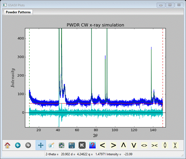
Again, I have used ‘+’ and zoomed in to show the interesting part of the pattern.
As additional work you can do sequential simulations to
explore the effect of changing probabilities. Try varying TransP;0;0, i.e. layer 1 –
layer 1 (CS) transition probability and TransP;2;1,
i.e. layer 3 – layer – 2 (HS) transition probability. Be sure the Symmetric probabilities box
is checked otherwise you’ll get nonsense. This ends this stacking fault
tutorial; the next one involves using kaolinite layers to simulate diffraction
patterns from kaolinite clays.